7.7.5. Comparing Predictive Performances

7.7.5. Comparing Predictive Performances

You can now compare the predictive performance of the global, local and DELTA models (global GLB_RLM_CLint, Local_RLM_CLint and DELTA_CLint, respectively).

1. If you have not yet done so, close ADMET Modeler and return to ADMET Predictor. Once in ADMET Predictor, calculate ADMET properties for all 51 unhidden compounds in the spreadsheet as described here. These should include Local_RLM_CLint, DELTA_CLint, and GLB_RLM_CLint as user attributes.

2. Compare the various predicted RLM CL_int values with the experimental values (OBS_RLM_CLint) by plotting them on a scatter plot (typically Chart 2). Clicking on the Chart Properties (1) icon in the Chart toolbar lets you set the axes appropriately.

1. Select GLB_RLM_CLint for the X-axis, OBS_RLM_CLint as the Y-axis, and put each on a log scale ranging from 1.3 to 3.7. Clicking on the linear fit icon on the chart toolbar (2) will post the linear fit statistics at the top of the scatter plot.

2. Add two more 2D scatter plots as described in Plotting Data. Select Local_RLM_CLint and DELTA_CLint as the X-axis for the respective plots; put OBS_RLM_CLint on the Y-axis for both. Click on the Linear Fit (2) icon in Chart 3 and Chart 4 to display the corresponding goodness-of-fit statistics.

   
   
   

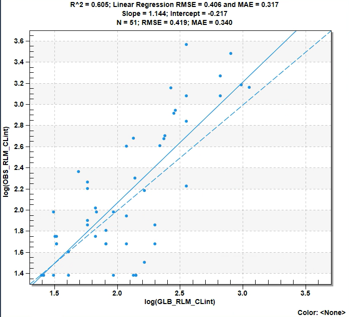
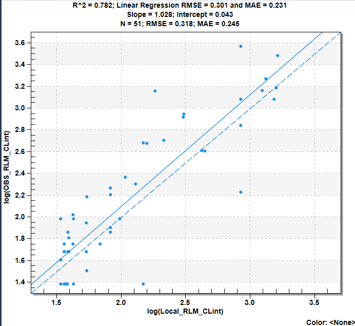
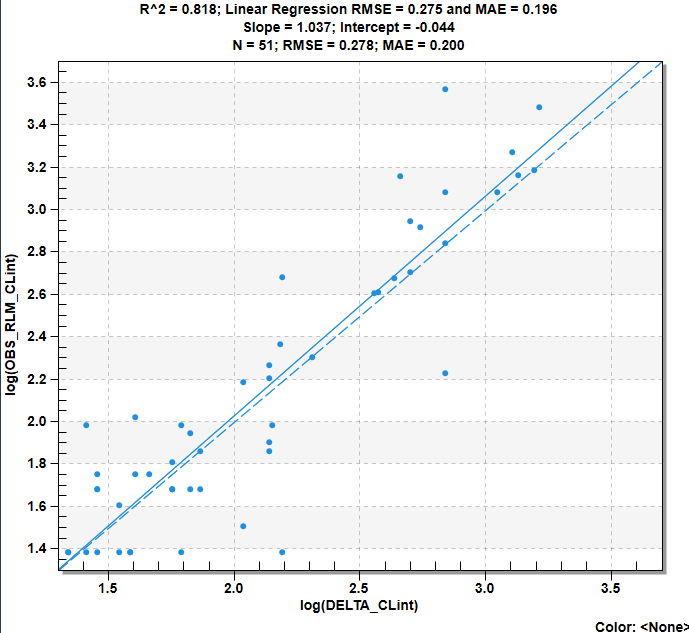
The three models exhibit different error patterns, but visual inspection suggests that Local_RLM_CLint outperformed the global model (GLB_RLM_CLint) on the full data set and that DELTA_CLint outperformed both. The RMSEs and MAEs bear this out quantitatively.

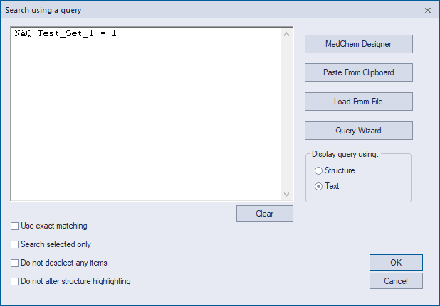
1. These statistics combine errors from the training pool and the test set. How well did each perform on the test set alone? Select the compounds assigned to the test set using EDIT >> Query By Structure/Property or by using the keyboard shortcut Ctrl+Q; either will launch the Search using a query dialog. Load the query shown below from Test_set_Selection.cqf to highlight those rows that belong to Test_Set_1.

   

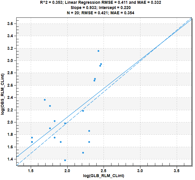
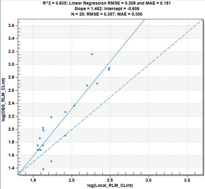
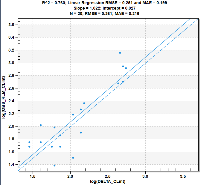
2. Twenty compounds will be selected. Hide the unselected compounds using VIEW >> Hide/Unhide >> Hide Unselected or the keyboard shortcut Ctrl+Shift+H. The three scatter plots described above and the associated correlation statistics will be updated automatically to focus on the 20 unhidden test set compounds.

   
   
   

3. The table below shows the predictivity statistics for the three models on the 20 compounds not used for model building or ensemble selection.

These numbers confirm that DELTA_CLint outperforms the other two ANNE models.

Note: This data set included several sets of stereoisomers, which is not particularly unusual in real-world drug discovery projects. In some cases, RLM CLint values for stereoisomers are similar, whereas for some others they were different. This can be handled, as was done here, by grouping stereoisomeric compounds together and then randomly assigning the groups to the training pool and test set - a "leave groups out" validation approach. Assigning the individual optical isomers independently would complicate interpretation considerably.