Regression Uncertainty

The connection between Bayes Theorem and regression uncertainty is less direct, mostly because it reflects the spread of a distribution of possible values rather than a single probability. The model training process is designed to make the predictive error itself 0 on average; it is the expected spread around 0 that is of interest. That spread of interest is generally the standard deviation σ_i,err of predictive errors for each ensemble prediction:

where σ_i,err is the population standard deviation of prediction errors for compound i, E represents the expectation across all small perturbations of the model, y_pred is the ensemble prediction, and y_obs is the experimentally observed value. Unfortunately, the ensemble model produces exactly one prediction for each input structure, which makes it impossible to calculate an estimate for σ_i,err (i.e., s_i,err) directly in isolation. It is possible to calculate s_i,err for the training pool and test sets used to train the model, but only because the true value of the dependent variable is already known in those instances. It cannot be calculated directly when making predictions for new compounds.

The standard deviation s_i,pred of the individual network predictions around their average, on the other hand, can be calculated for any prediction:

where y_ij are the individual network predictions, y_pred is the ensemble (average) prediction, and k is the number of networks in the ensemble. Moreover, it is reasonable to expect that s_i,pred reflects the underlying predictive uncertainty. Beck et al. (2000) noted that s_i,pred varies considerably from compound to compound and that it is an overly optimistic estimate of the standard deviation of the ensemble predictive error (s_i,err). They opted to distribute the missing (residual) error across compounds in proportion to s_i,pred, scaling up each by a constant γ:

The justification for such uniform scaling is shaky at best, given their acknowledgment that the predictive uncertainties are different for different compounds. It is in principle subject to rigorous statistical testing, but the large secondary test sets needed to validate the error model are hard to come by. That is especially true when the uncertainty model has to be trained on the primary test set used to construct the model.

The calculus involved in getting from Bayes Theorem to our regression uncertainty analysis method is beyond the scope of this document. It will be discussed in detail elsewhere (Waldman et al., in preparation) but the upshot is that s_i,err is calculated as follows:

Cumulative gamma distributions F and G that share two parameters - β and s₀ - are fitted simultaneously:
1. F with parameters α_err and β is fitted to the distribution of err² across s_i,pred-s₀ by minimizing the Kolmogorov-Smirnov statistic, i.e., the maximum deviation of the observed cumulative from the predicted cumulative.
2. G with parameters α_pred and β is fitted to the distribution of s_i,pred-s₀.
The standard deviation of the predictive error is estimated from the corresponding probability density functions f and g:

The shared parameter β determines how rapidly the gamma distributions fall off. The common offset (s₀) allows for the fact that, as a practical matter, the spread in network predictions does not go to zero, though the "pure" distributions may. The need for it may also reflect the effect of experimental error in the data the model is trained on, but this is a matter for further investigation.

That the contingent error distribution g(s_i,pred) can be well-fit by a gamma distribution is fortunate. The gamma distribution is a generalization of the chi squared distribution, which is followed by the squared standard normal deviate (the normal deviate divided by its standard deviation σ). It is generalized in the sense that α can only take on half-integer values and β = 1/2 for the chi squared distribution, whereas both parameters are free to take on any positive value for gamma distributions.

If the predictive errors are normally distributed and s_i,err is an accurate estimate of σ_i,err for all compounds, then all normalized errors (err/s_i,err) can be expected to follow the standard normal distribution and their squares will follow a gamma distribution. Having that be the case to a good approximation makes calculating confidence intervals and identifying significant differences straightforward.

Pairing a gamma distribution for F with a gamma distribution for G that has the same β parameter makes the ratio of the two monotonically increasing in s_i,pred - provided α_err ≥ α_pred for the fitted distributions. There is nothing intrinsic to the process that guarantees this will be true, but uncertainty models for which α_err < α_pred are unrealistic and pathological. Hence they are discarded automatically by the program.

One might expect that the prediction variance s_i,pred² would also follow a gamma distribution, but it does not. The standard deviation of prediction (s_i,pred itself) does, however; at least it does to a good approximation for the data sets we have investigated to date. When that is true, s_i,err calculated as described above appears to be a good estimate of σ_i,err. The accuracy of the estimate sometimes breaks down when s_i,err gets large, but predictions with the large uncertainties that result should probably be discounted anyway.

Plotting cumulative distributions

The relative cumulative distribution of the squared error err² as a function of s_pred is determined as follows.

Calculate err² for each point.
Index the predictions in increasing order of their s_pred value.
For a given k, sum the squared errors for all predictions whose ensemble standard deviation is less than or equal to that of prediction k, then divide this sum by the total squared error to yield (relative) cumulative squared error prediction:

where ERR_k is the relative cumulative squared error of prediction k. The sum in the numerator runs over all errors for which the ensemble standard deviation is less than or equal to s_k,pred, while the sum in the denominator runs over all errors.

The correction factor of N/(N+1) is analogous to the continuity correction used for CFA calculations. Problems arise if it is not applied, because unity is only reached at infinity for the theoretical distributions of interest but is necessarily reached for the Nth point in the formula given above if the correction is omitted. Other choices are possible for this correction, and there is a substantial literature devoted to the topic of how to choose “plotting positions.”

As of ADMET Modeler 10.4, the cumulative distribution of ensemble standard deviation for a given data point is calculated by counting the number of points with an ensemble standard deviation less than or equal to the point in question and subtracting 0.5 from this value. This quantity is then divided by the total number of data points. This is usually referred to as the Hazen formula in the statistics literature. This correction to the plotting position is similar to that used for the continuity correction for classification models. Internal testing found this to provide a small improvement to the use of the N/(N+1) factor that had been previously used, because the values at the extremes are not as close to zero and 1 (assuming N is reasonably large) and leads to improved fitting of the distribution. This formula is also used in generating the QQ plot for normalized error. The formula cannot be applied to the squared error distribution, because the cumulative squared errors are continuous quantities rather than discrete counts of points.

Quantile-Quantile (Q-Q) plots

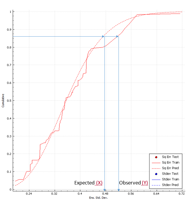
Given two cumulative distributions, F and G, let F^-1 and G^-1 be their inverse cumulative distribution functions. In our case F and G are functions of the ensemble standard deviation. Let y_i be the observed ensemble standard deviation for a given point. Let G(y_i) be the observed cumulative distribution (err² or s_pred as described above) for point i. Then, let x_i = F^-1(G(y_i)) where F is the fitted or theoretical cumulative distribution. For each point i, determine its x_i and y_i values and create a graph of these points. The x axis is conventionally labelled as the “Expected” value of the argument of the distribution function (ensemble standard deviation in our case) and the y axis as the "Observed" value. If the theoretical/fitted cumulative distribution perfectly fits the observed cumulative distribution these points will lie on a straight line with slope 1 and intercept 0. This ideal fit is shown as a dashed line on the Q-Q Plot.

A way of visualizing the construction of these points is to work from the cumulative distribution plot as in the example shown below. Starting from a cumulative distribution value of 0.85, one draws a horizontal line to both the theoretical distribution and the observed distribution. At the intersections to this line, one drops vertical lines to the X axis representing the ensemble standard deviation. The X coordinate of the vertical line coming from the theoretical distribution is the expected value of the ensemble standard deviation; it becomes the X coordinate on the Q-Q Plot. The X coordinate of the vertical line coming from the observed distribution is the observed value of the standard deviation; it becomes the Y coordinate of the Q-Q Plot. Thus, deviation of points from the diagonal line on the Q-Q plot is a measure of the horizontal separation of the two cumulative distributions. This is a useful measure, as the theoretical distribution was fitted by minimizing the Kolmogorov-Smirnov statistic, which is a way to minimize the vertical separation between the two graphs. Visualizing the deviations of their horizontal separation provides a measure of how well the fit performed.