

3.4.1. Modeling Methods
ADMET Modeler supports four different model-building methods: Artificial Neural Network (ANN), Support Vector Machine (SVM), Multiple Linear Regression (MLR) and Kernel Partial Least Squares (KPLS). All four can be applied to numerical dependent variables, but only ANN and SVM can be applied to categorical variables where at least one class label is textual. ANN and SVM classification models can now handle up to 16 distinct class labels. All are proven tools in machine learning and artificial intelligence; details of their workings are given below.
Artificial Neural Networks (ANN)
ANNs can model complex nonlinear relationships without requiring a priori knowledge of the underlying mechanisms relating descriptors to the property of interest. Because nature is not piecewise linear, or even piecewise nonlinear, we believe ANNs offer one of the most powerful methods available for modeling structure-property relationships.
The process of training an ANN begins with a random set of coefficients (weights) that are then adjusted (optimized) to better fit the data. The disadvantage of any single ANN (and of most other modeling methods) is that it may find a “local minimum,” which is one of any number of possible solutions, based on a particular architecture. Here, architecture refers to a particular combination of neurons and inputs in an ANN. Different initial random coefficients often result in different final models. Where you start can determine where you finish, as is the case in most optimizations. Modeler builds many candidate models, then picks those which perform best and combines their predictions. This makes it likely that the networks in the ensemble will be ones that lie reasonably close to the global minimum and that their aggregate predictions will be accurate.
An artificial neural network is a connected set of mathematical functions. For each descriptor (or input), a coefficient (also called a “weight”) multiplies the value of the descriptor and that product is sent to a neuron (also "unit" or "node"). The neuron sums the inputs and subtracts a threshold weight as a bias term. This resulting number is used by an activation function to generate the output of the neuron. ADMET Modeler uses a hyperbolic tangent function for activation.
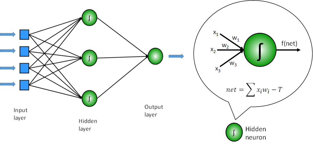
ADMET Modeler uses only one layer of neurons between the inputs and the output. This layer is called the "hidden" layer because it is between the inputs and the output. Some artificial neural network models use multiple hidden layers; however, our experience is that a single hidden layer is sufficient for most problems and tends to be more robust than more complex architectures.
The output of each neuron is multiplied by a weight and sent to the final output neuron, which sums the outputs of all hidden layer neurons and subtracts a final output threshold value (weight) to obtain a numerical output. For regression models, that value is the prediction. For binary classification models, a logistic function is applied to the output. If the resulting value falls above an optimized threshold, it is classified as a positive; otherwise it is classified as negative. "Training" the ANN consists of adjusting the set of weights so as to minimize the sum of squared errors for the training set. In the case of ANNE classification models, the sum is a weighted sum of squares. For multi-class classification models, each network outputs multiple logistic function outputs, one output corresponding to each class. The output class with the largest output becomes the model prediction. In this case, the sum of squared errors is done over all classes for a given observation where the target value is 1 for the observed class and 0 for the other classes.
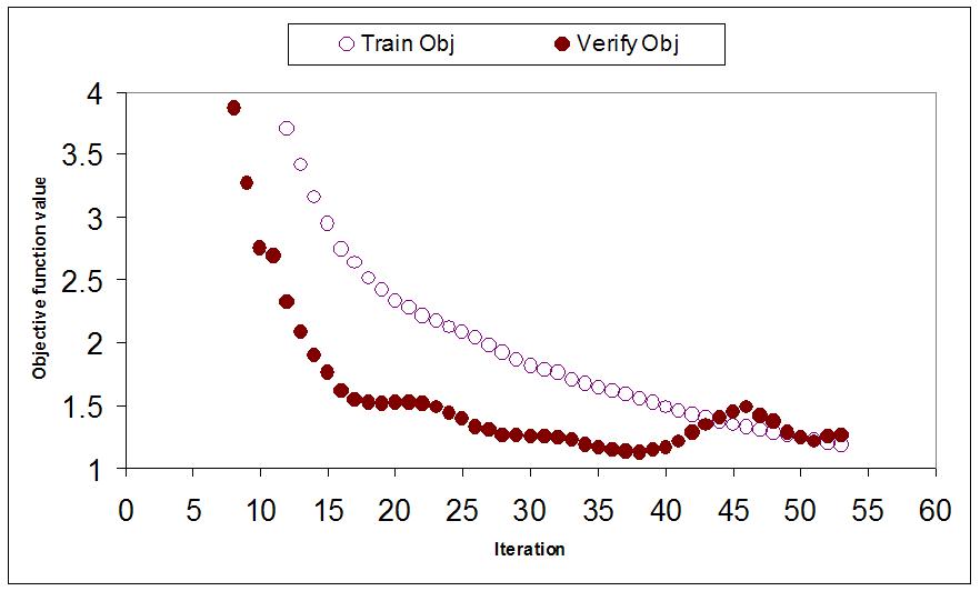
We use early stopping to guard against ANN overtraining. This is done by applying an iterative optimization process to the training set while monitoring the accuracy of predictions made on the verification set. Training terminates once the model loses generality – the ability to predict properties for compounds that are not in the training set. The objective function is the RMSE for the training set, which necessarily decreases every time the model weights are adjusted. The verification set RMSE also initially decreases, but the verification set RMSE eventually begins to increase because overtraining occurs as the model starts to fit noise in the training data. At the point when the verification set error fails to improve or increases for more than a specified number of iterations, training is stopped and the coefficients from the iteration at which the minimum verification RMSE was achieved are used for the model.
See Section 3.4.2 for details on how the individual network outputs are combined to produce an ensemble output.
Linear Boost Networks (LBN)
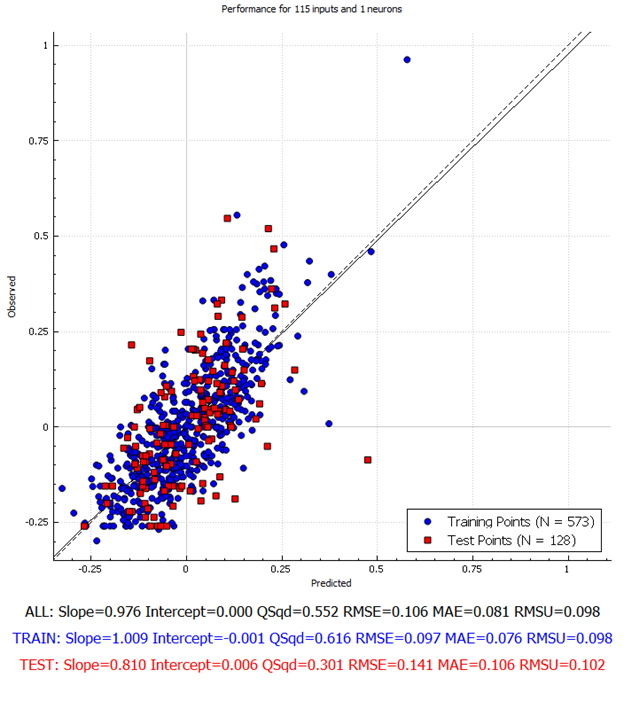
Sometimes ANN models’ output range is “squeezed”, i.e. much more limited than the observed range of its dependent variable, especially when trained on data with poor signal-to-noise ratio. An example of this phenomenon is shown below.
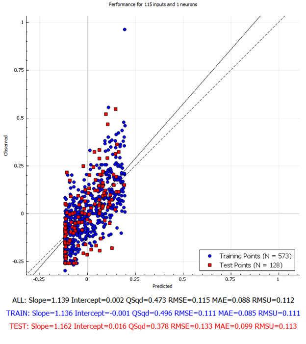
The range compression is not unexpected considering sigmoidal activation functions employed in hidden neurons. Sometimes adding more neurons helps alleviate this problem, but we came up with a new ANN architecture that by its very nature has an unlimited range. It is called a Linear Boost Network (LBN) and illustrated in the figure below:
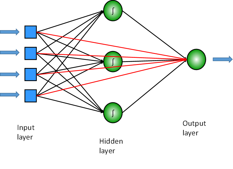
It is similar to the ordinary ANN from previous section with one exception: it features an extra set of weights that directly connect input and output layers (red lines). It could be interpreted as a merger of ANN and Multiple Linear Regression (MLR) models. Its effect on the same troublesome data is shown below - output range compression is gone.
Currently, LBN is available for regression models only and can be activated by clicking a check box in Artificial neural network settings.
Support Vector Machines (SVM)
The most recent advance in machine-learning to find widespread use outside of artificial intelligence itself is the support vector machine. First developed by Vapnik in 1992, the SVM is an outgrowth of kernel methods. In such methods, the data is transformed with a kernel function (e.g., a radial basis function) and it is in this transformed space ("kernel space") that the model is built. Care is taken in the construction of the kernel that it has a sufficiently high dimensionality that an underlying linear relationship can be found within it. A subset of transformed data points - the set of “support vectors” - is then used to specify a hyperplane that effectively serves as a linear model within this space. An introductory exploration of SVM is provided by Cristianini and Shawe-Taylor (2001) and a thorough examination of their mathematical basis is presented by [Smola and Schölkopf (1998)].
Our implementation uses the open source LIBSVM library developed by Chang and Lin (2011) following the work by Fan et al. (2011). If the number of classes k exceeds three, k*(k-1)/2 pairwise submodels are built for each individual SVM in the ensemble and which class gets the most submodel votes determines the class assigned to an observation by that individual SVM. See Section 3.4.2 for details on how the individual SVM outputs are combined to produce an ensemble output.
One potential advantage of SVM is that the objective function has, in theory, a single minimum, so the system cannot be trapped in a “local minimum” as other model building systems can. In addition, it has a built-in parameter designed to avoid overtraining. Nevertheless, an SVM can be over-fit if it is nonlinear or it is built on a data set that is too small or too noisy. Hence, in practice, an external test set needs to be set aside for validation, and doing so often demonstrates that an SVM is indeed over-trained. Typically, if the number of support vectors required by an SVM model is large relative to the number of training set compounds, you should seek more data or more informative descriptors or both.
SVM does outperform ANN in optical character recognition applications (Russell 1995). In our hands, however, applications of SVM to the prediction of ADMET properties from molecular structure does not reliably improve overall performance versus that seen for our ANNEs.
Kernel Partial Least Squares (KPLS)
KPLS was first introduced by Rosipal and Trejo (2001). It is a relatively new member in the family of regularized least squares regression methods that incorporates the kernel method described above for SVMs into the Partial Least Squares (PLS) paradigm that is popular in the field of chemometrics (Wold 2001).
The basic idea of KPLS is to build linear PLS models in a non-linear space. Each input point in primal space is mapped into a higher-dimensional (possibly infinite) kernel space, also called feature space. A linear regression function is constructed in the feature space using the PLS algorithm, corresponding to a non-linear function in the primal space.
Our implementation of KPLS requires optimization of two special parameters: a kernel parameter and the number of latent variables to use (Bennett 2003). The kernel parameter controls the non-linear mapping while the number of latent variables indicates the model complexity. For the RBF kernel, the larger the kernel parameter is, the smoother the model function will be. Model complexity increases when more latent variables are used in much the same way ANN complexity increases with the number of neurons.
There are two ways to determine the number of latent variables: one is tuning against a validation set and the other is to use a fixed value. To better automate this process, we have adopted the former approach. The program will automatically find the optimal number of latent variables. However, users may provide a range for the optimization of the kernel parameter.
KPLS and other kernel methods are inherently inefficient when applied to large data sets. Because the kernel matrix is NxN and has to be held in memory, it is very memory-intensive for large data sets. For example, the kernel matrix for a 10,000 points data set would take up to 400 Megabytes memory, even when full advantage is taken of matrix symmetry. Our experience indicates that it provides similar performance to ANN and SVM but is faster. KPLS may be worth trying first for non-linear modeling of moderate-sized data sets (\< 3,000 points).
Multiple Linear Regression (MLR)
Multiple linear regression assumes that the dependent variable (output/response/activity) is linearly determined by many independent variables (inputs/descriptors). The task is to find the linear coefficients between them. (Mayers 1989)
If the data set is well-behaved (i.e., if the inverse of the covariance matrix of the inputs exists) the solution of the linear coefficients can be obtained directly by linear algebra. However, many real data sets are not well-behaved and simple linear algebra will not work well.
MLR is worth trying when you know the underlying relationship is linear or the data set is small and relatively few descriptors are being considered. Small data sets often do not contain enough information to build a robust non-linear model, but you can build MLR models with any data set. It is fast and (usually) provides an indication of minimum fitting performance you can expect from the other methodologies implemented in ADMET Modeler. It is the approach least prone to overtraining, provided the number of observations is several times (e.g, 5-7) times larger than the number of descriptors used.
XGBoost (eXtreme Gradient Boosting, XGB)
In version 13 we have added code to read and run eXtreme Gradient Boosting (XGBoost) ensemble models in ADMET Predictor. A single XGBoost model is a collection of progressively boosted decision trees (Chen 2016). This modeling technique gained widespread recognition as a winner of many Kaggle competitions. ADMET Modeler is NOT yet capable of training such models. Both regression (RXGB) and classification (CXGB) models of this type must be built using external software. Currently, only binary classification XGB models are processable by ADMET Predictor. We used Python scripts developed in house to build the few XGB models distributed with the program. The format of each contributing XGBoost model is standardized by the Python's 'xgboost' library as either .json or .ubj file. Both of these formats are recognized by ADMET Predictor. These are collected into an ensemble using the .xgb file format developed at Simulations Plus and described in the FILE FORMATS appendix.