3.4.8. Composite Models

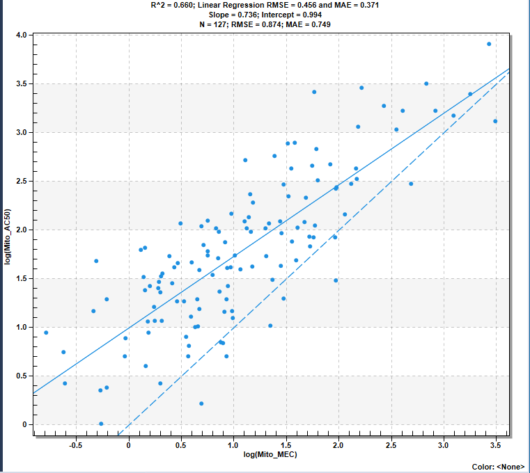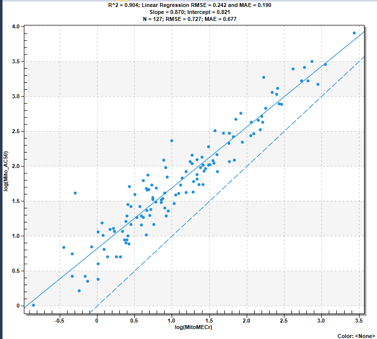
Sometimes the modeled endpoints are mutually dependent via either equality, or inequality constraints. The classic example are the Michaelis-Menten constants of metabolic transformation, V_max and K_m, constrained by the related intrinsic clearance definition: CL_int = V_max / K_m. A newer example are the most recent models (ADMET Predictor 14) of apparent permeability across Caco-2 and MDCK-MDR1 cell monolayers. In the latter, the efflux ratio, ER, is tied to the observed apical-to-basolateral, AB, and basolateral-to-apical, BA, permeabilities: ER = BA / AB. DILIsym module models of mitochondrial dysfunction and reactive oxygen species serve as an example of inequality constraints: experimental design requires the MEC < AC₅₀ relationship at all times. In all cases there are independent data sets containing separate measurements of all the mentioned endpoints. One can simply build direct QSAR models of each endpoint separately, AB, BA, and ER for example, and present these to the end user. Having done exactly that with models of V_max, K_m, and CL_int many years ago we have encountered quite a few complaints from our customers: “Predicted values do not satisfy the CL_int = V_max / K_m relationship!” No surprise here, independently developed direct models cannot possibly be expected to “know their place” and follow arbitrary mathematical formulas. On the other hand, if the said endpoints were measured for a given compound in the same experiment, then they should be related to each other as expected.

We have developed methods guaranteeing satisfaction of the mentioned relationships for all predictions. It is not a secret that one equality constraint lowers the number of independent variables in, e.g., apparent permeability models from three to two. Hence, a projection of the related 3-dimensional space onto a 2-dimensional subspace that is orthogonal to the constraint would automatically satisfy the latter. But how to do it for a nonlinear constraint? Fortunately, logarithms come to the rescue:

The constraint is thus made linear and we can happily apply linear algebra. The 2D subspace orthogonal to this constraint is a 2D plane orthogonal to the [1 -1 1] vector. It is good to normalize it into the following unit vector to avoid scaling issues:

The 2D plane orthogonal to this vector is illustrated below:

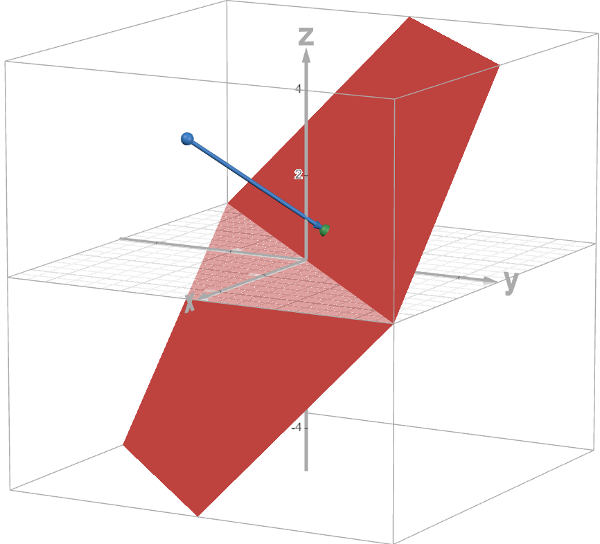
It is not difficult to find two other unit vectors that along with the above vector form an orthonormal basis set of the 3D space. Putting all three into a matrix acting on the vector of logarithms of permeability endpoints yields a vector of two independent, orthogonal components X and Y:

The above transformation is used to generate “observed” values of the X and Y components with eventual (and hopefully rare) gaps filled with predictions of independent QSAR models of log(ER), log(BA), and log(AB). ADMET Modeler is then used to build independent models of X and Y. Since the transformation matrix is orthonormal its inverse is easily obtained by transposition. Acting on the vector of X and Y predictions the inverse allows for calculation of the properly constrained predictions of the original endpoints:

For a curious reader, the determinant of the two transformation matrices is equal to +1, thus they represent rotations of the 3D space.

It is worth mentioning that the reconciliation strategy for atomic level models described in the section on CYP enzyme kinetics is also a linear transformation in the log space:

Unlike for the distance-preserving rotation, however, the above singular matrix represents an oblique projection onto the plane along the [1, -1, 0] direction.

Dependent models that are expressible as linear combinations of independent models, like the apparent permeability, AB, BA, and ER, are designated by the special COMB type and encoded in a .cmb file described in the FILE FORMATS appendix.

Finally, to prevent non-physical predictions where MEC > AC₅₀ for the DILIsym models mentioned above, an independent direct model of better defined AC₅₀ is developed in the log space first, log(dAC50). Next, for all compounds with both properly measured MEC and AC₅₀ the following relationship must hold:

AC₅₀ - MEC > 0

Therefore

r ≡ MEC / AC₅₀ < 1

This relation is used to calculate the “observed” ratio values, r, from which a QSAR model is subsequently developed in logit space, Z = logit(r). When an AC₅₀ value is not available, then it can be replaced by the dAC50 prediction, but only if the above relation holds. Finally, the predicted MEC is calculated from:

Recall that and which is always guaranteed to be between 0 and 1. In practice, one exports the Z model with dAC50 specified as both the Auxiliary Factor and the Determining Descriptor in Model Editor, for example:

The former takes care of the multiplicative scaling, the latter informs the Z model that the dAC50 is a critical dependence it can’t run without.

For illustration, we have taken the training data of AP12 Mito_AC50 and Mito_MEC models and built the MEC/AC50 ratio model in logit space (using the AP15 aggregated atomic descriptors). The best model has been exported (MitoMECr) as illustrated above. As expected, the constrained model’s performance is slightly worse than that of the original Mito_MEC:

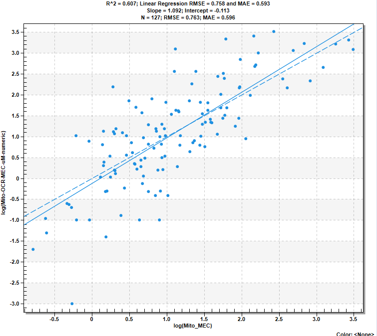
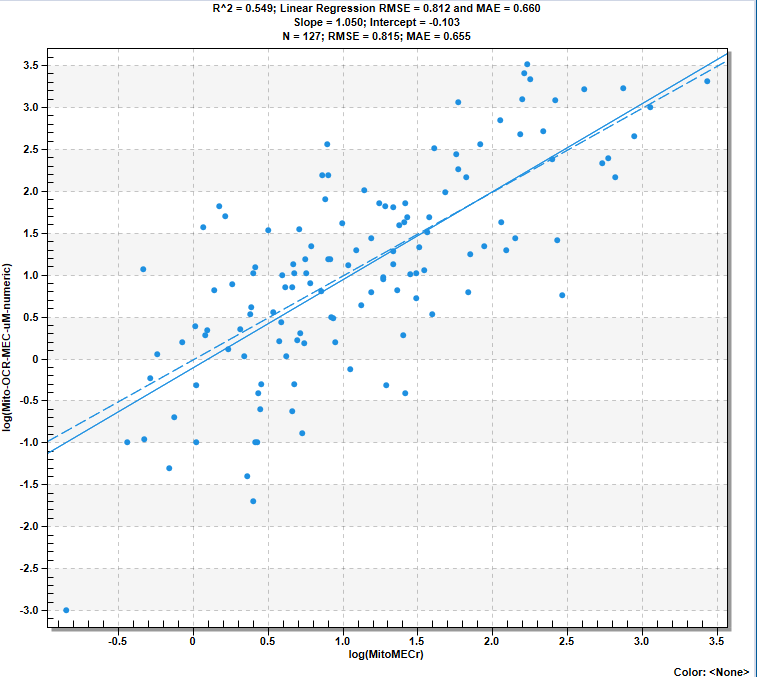
The advantage of the latter is the guaranteed MEC < AC₅₀ relation for all predictions, as designed: