5.2.1. AIDD Theory

The AI Drug Design module uses a multi-objective evolutionary algorithm based on Pareto or MCDA optimization to grow a library of molecules optimized against multiple criteria starting from one or more seed molecules. An outline of the algorithm is shown in the workflow chart below.

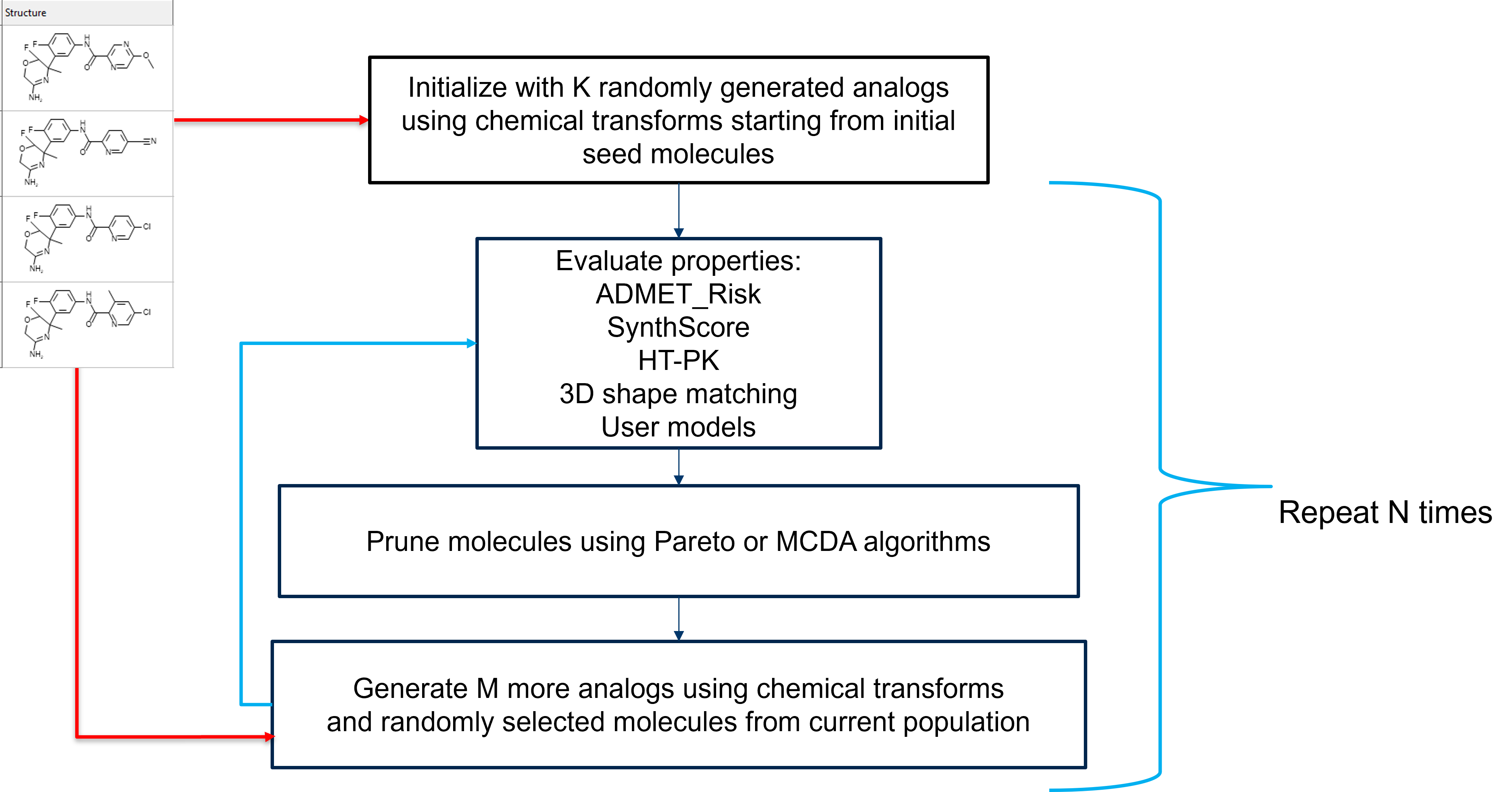
The parameters K, L, M, and N correspond to the user-specified Run parameters, “Size of initial population”, “Minimum size of population after each pruning cycle”, “Number of candidate molecules per generation”, and “Number of optimization generations”, respectively. Each of the above steps will now be described in detail.

When an AIDD run begins, all selected molecules in the spreadsheet are automatically added to the initial population of candidate molecules. The program then attempts to add additional molecules until the starting compound population meets the required number specified by the Size of initial population parameter. Additional candidate molecules are generated as follows. First, each molecule in the population is assigned a weight. Initially, all molecules have equal weights. If a given molecule generates a “child” molecule, its weight is lowered, so as to reduce the chance that it will generate additional child molecules. This helps to maintain chemical diversity in the population and avoid having one parent molecule generate too many children. After the weights are assigned, a parent molecule is selected randomly from the current population with a probability proportional to its weight. Next, a reaction transform is selected randomly from the list of available transforms provided in the Input file containing transform rules. Any transforms that have been disabled are omitted from the list of available transforms. Using the selected transform and parent molecule, the program generates all possible products from that parent/transform combination. As a trivial example, if the parent molecule was propane, and the selected transform was Add_chloro, both 1-chloro and 2-chloro propane would be generated as product molecules. Each product molecule is checked to see if it passes the Scaffold query (if specified) and passes all filter criteria (if specified). Each product molecule is also checked to make sure it is not in the current population nor is it a molecule whose properties have already been evaluated. From the list of product molecules that survive these screens (if any), one of them is randomly selected and added to the current population, and the weight of its parent molecule is updated (decreased) since one of its children has been added to the population. This process is then repeated (i.e., random selection of a new parent molecule and randomly selected transform) until the required number of initial molecules is generated. The program keeps track of any parent molecule/transform combinations that fail to generate new product molecules, so that combination is never tried again. In the unlikely scenario that all parent/product combinations fail to generate the required number of candidate molecules, then the program will resort to trying reaction transforms two at a time (similar to the Combinatorial transforms feature).

Once the initial population size has been reached, all molecules are submitted for property evaluation. Calculation of ADMET properties and molecular descriptors is automatically performed. If %Fa or %Fb has been selected, then HTPK simulations are also performed. Any target property corresponding to an ADMET Model that is out-of-scope for a given molecule is then penalized by adding (for minimized properties) or subtracting (for maximized properties) the out-of-scope penalty to the calculated value. Any Risk model is also penalized based on the risk out-of-scope factor. See the discussion about the Risk out-of-scope penalty for more details.

After all the target properties have been calculated, the population is then pruned based on Pareto selection. The selection proceeds by finding all molecules that are “dominated” by at least one other molecule in the population. A molecule is considered dominated by another molecule if it is inferior in at least one objective and is not superior in any objectives. In mathematical terms, consider molecules (represented as points in a multi-dimensional space of the objectives) p and q with n properties, p_i and q_i, i = 1, …, n. Then, p dominates q if there exists at least one property j such that p_j \< q_j and there is no property k such that q_k \< p_k.

This assumes the properties in question are being minimized. If a given property is being maximized then the inequality would be reversed for that property. All dominated molecules are then removed (pruned) from the population, and the remaining molecules are considered Pareto optimal. In other words, there are no molecules that dominate them. Graphically, this may be illustrated in the following two-dimensional example:

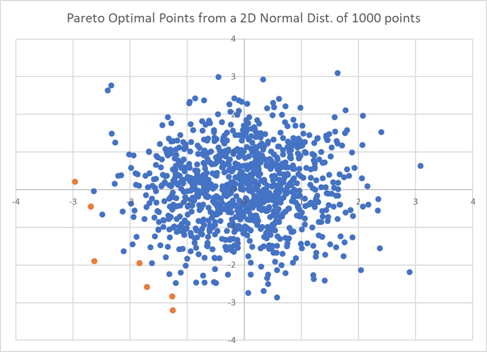
The points above were generated from a random selection of points following a normal distribution along each dimension. The amber-colored points represent the Pareto optimal subset (assuming the objectives are being minimized). Of the 1000 points, only 7 are Pareto optimal. These 7 points dominate the remaining points in the set and are said to lie on the Pareto front. Typically, as the dimensionality of the space (number of objectives) increases, the percentage of points on the Pareto front increases because more of the space is located near the surface. For example, conducting the same experiment as above but with a 5-dimensional distribution of points found ~100 out of 1000 points as Pareto optimal. In-house testing with various AIDD runs generally finds more objectives (target properties) leads to more molecules in the final solution. Consequently, to provide a reasonable limit to the number of generated molecules, the program currently limits the total number of selected properties to five. Even with this setting, a very long AIDD run (~10,000 generations) can lead to tens of thousands (or more) of product molecules which are all Pareto optimal.

After pruning, if the current population is smaller than the “Minimum size of population after each pruning cycle” setting and the number of generations has reached 100 or one half of the total number (whichever is smaller), then additional molecules will be selected from the ones that were pruned by re-applying the Pareto selection strategy to the pruned molecules (while omitting the already selected molecules from this list). This approach is known as selecting multiple layers of Pareto optimal points. (Liu, 2019) An illustration of the approach using the above distribution of points is shown below.

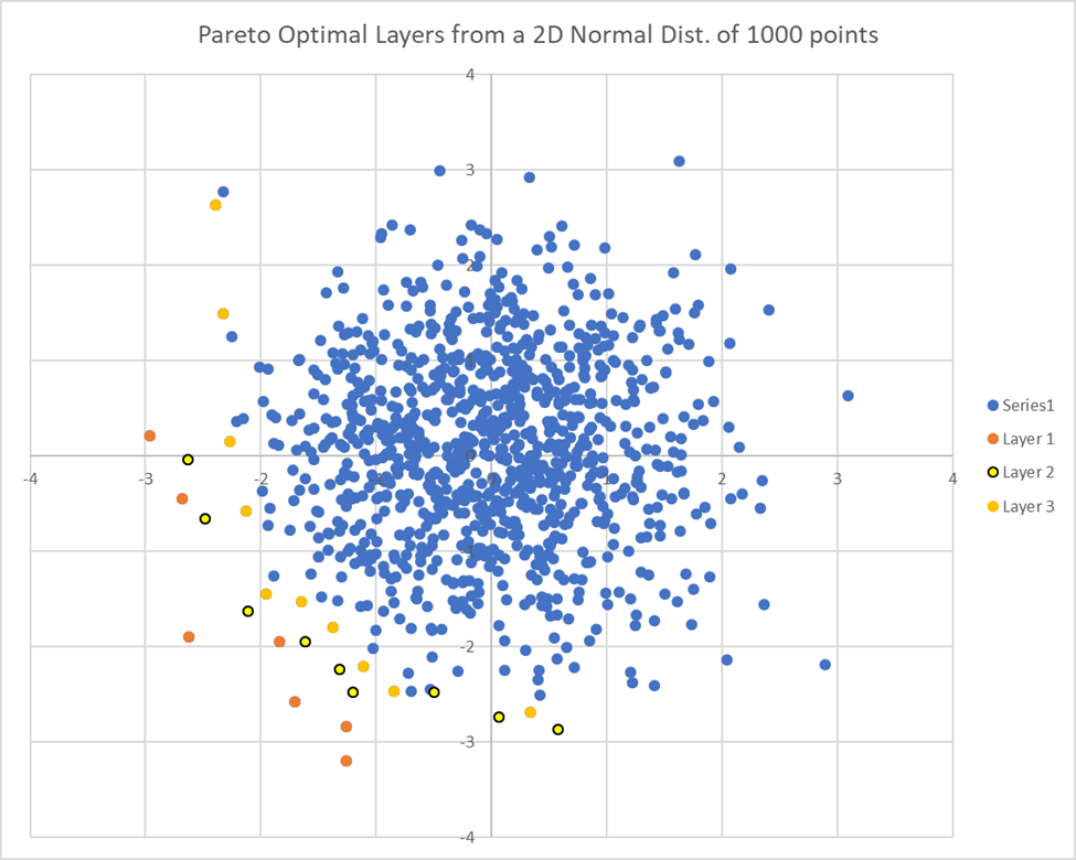
Here, the points selected from the first 3 Pareto optimal layers are shown. Points will be selected from each successive layer until the minimum required number of points criterion has been met. The reason for not imposing this constraint until midway through the run is to allow the initial population to grow gradually with “good” (Pareto optimal) molecules. This generally leads to faster convergence and a better overall solution. Also, note that the pruning step may result in a decrease of the total population from one generation to the next. This can happen if a new candidate molecule dominates multiple molecules in the current population causing them to be removed upon pruning.

After the pruning step has completed, all molecules remaining in the population are assigned new weights (for the purpose of prioritizing them for product molecule generation). The weights are based on the number of children produced by a given molecule, its Pareto layer count, and its Borda Rank (sum of ranks across all objectives). See the discussion on Finding the Best Ensemble for a detailed description of the Borda Rank statistic. More children lead to a lower weight (so as to reduce the likelihood of this molecule being selected to generate another analog) while a lower layer count and a lower Borda Rank lead to a higher weight as the molecule is deemed better in terms of its properties. The current population is then used to generate M additional candidate molecules (as shown in the workflow diagram above) using the exact same protocol involving selection of a parent molecule and reaction transform as was used to generate the initial population. These candidate molecules are then submitted for property evaluation, followed by another pruning of the total population, and so on. The overall process is repeated N times corresponding to the Number of optimization generations specified for the run.

ADMET Predictor offers also an alternative to described above Pareto-based pruning. Often, it useful to treat the objective functions with various priorities/importances. To achieve this, the user can utilize the Multicriteria Decision Analysis (MCDA) pruning method, which, instead of analyzing Pareto frontiers, calculates the ranking of the molecules and passes only the most valuable individuals to the next generation. The MCDA pruning implemented in ADMET Predictor uses the well-established Vikor (VIšekriterijumsko KOmpromisno Rangiranje) method. This method is a multi-criteria decision analysis (MCDA) technique designed to rank and select from a set of alternatives based on multiple conflicting criteria. It focuses on identifying a compromise solution that is closest to the ideal, accounting for the best and worst performance in each criterion. The method calculates a utility measure and a regret measure for each alternative, which are then combined into a single VIKOR index. This index is used to rank the alternatives, highlighting the option that provides the best trade-off between criteria.

VIKOR is particularly useful when decision-makers need to find a balance among conflicting objectives. The implementation in ADMET Predictor allows the user to assign a weight to each considered objective function. These weights, together with information about the preference direction and the objective function values, are passed to the VIKOR algorithm, which returns a ranking expressed in terms of integer numbers. In a given iteration, a portion of highly ranked molecules is passed to the next iteration, where the portion reflects the fraction of iterations completed so far.

As of the release of version 13, the Synthetic Difficulty calculation (S+SynthDiff) has been replaced with the SynthScore model. Along with the DrugLikeFilters that are applied by default in the Filter rules, use of the SynthScore model will skew the evolution of molecules toward more realistic structures, reducing the number of molecules that are undesirable from a synthetic chemistry perspective. It is important to note that the SynthScore is only a prediction of synthesizability based on retrosynthetic analysis and ultimately needs to be assessed by a synthetic/medicinal chemist.

Capping Values: Pareto or MCDA-based selection can often find molecules that are good in just one property and poor in all (or most) other properties. If the value of the “good” property is among the best in the population, it may be difficult to find another molecule that dominates it, so it will tend to remain in the population. In early experiments, we attempted to cull such molecules out of the population by removing molecules which were in the bottom X% of a given property (typically 10%). However, this turned out to lead to poorer overall results in the final population as some of the better molecules in the final population were no longer found. The reason for this result is that molecules that are poor in just one property but good in most others have a reasonable chance of generating an analog that improves the one poor property while maintaining the good results for the other properties. Culling such molecules from the population can lower the likelihood of finding their “improved” analogs. On the other hand, molecules with many bad properties but just one good property have a much poorer chance of leading to an analog that has desirable behavior across the broad spectrum of properties. Such molecules can be “weeded” out of the population by a protocol which assigns a Capping Value to that property. Employing this strategy generally results in final populations with better overall property values. Experience with Capping Values suggests a Capping Value for %Fa or %Fb in the range 80-95 and ADMET_Risk in the range of 1.5-2.5 leads to good results, while preventing a very good score in either of those objectives from allowing otherwise “bad” molecules from remaining in the population. Capping Values for other properties or user models (such as an activity model) need to be explored by analyzing results using different values with several AIDD runs. Ultimately, the user needs to decide at what point a given property is “good enough” (which should be its assigned Capping Value) and the Pareto selection strategy should then focus on other properties when comparing molecules. Note that if a Capping Value is assigned to a given property, then that will be the value shown in the OBJ_* column for that property if the Capping Value is applied to a given molecule. The actual value for the property can be found from the corresponding ADMET/HTPK column in the final spreadsheet or by running ADMET/HTPK calculation on any of the intermediate smi files.