

5.2. AI Drug Design
The AI Drug Design Module enables users to generate candidate molecules optimized against multiple objectives via an iterative procedure starting from one or more seed molecules that are modified via SMIRKS transformations (similar to Combinatorial Transform) and evaluated against the multi-objective targets. Incorporation of objectives such as ADMET Risk™, and the use of out-of-scope penalties provides a means to reduce the frequency of “problematic” molecules often seen in compounds generated by computer algorithms (i.e. “de Novo design”). Additionally, the capability to define a scaffold as well as filters to block undesirable functional groups helps to limit the algorithm from exploring undesirable regions of chemical space. Finally, including HTPK objectives allows for the targeting of good pharmacokinetic properties in the resulting compound library. Thus, the module leverages many of the capabilities of ADMET Predictor into a flexible streamlined protocol for rapidly generating virtual molecules simultaneously optimized against multiple target objectives.
The user interface to this module is provided through a series of dialog boxes in the form of a “wizard”. After selecting one or more molecules in the current spreadsheet, the AI Drug Design wizard may be invoked from the menu via
Chemistry >> AI Drug Design or
Design >> AI Drug Design or
via the AIDD icon in the main ADMET Predictor toolbar:

Selecting either the menu command or the icon launches the first dialog, Compound optimization, of the AIDD wizard.
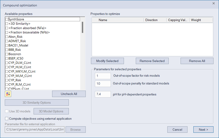
The list of Available properties on the left includes all models which output a numerical value (e.g., regression models, PLS models, Risk models), the HTPK properties, and 3D similarity to one or more reference structures (described below). Also included are specific tissue specificities, calculated from the species-specific tissue partition coefficients returned from HTPK simulations. User-built regression models (e.g., to model activity or inhibition) from ADMET Modeler may also be incorporated once they have been exported from ADMET Modeler to ADMET Predictor. All such user models are also included in the list. However, models that have been turned off in Model Editor will not appear in this list. One may select up to 5 objectives which will appear in the list of Properties to optimize. Either %Fa or %Fb (but not both) may be selected as part of these 5.
Internal testing has found that 5 is a soft limit for the number of objectives that can be simultaneously optimized effectively using either the Pareto or multi-criteria decision analysis (MCDA) algorithms, which are described below. Of course, there is no requirement to use all 5. Multiple criteria may also be combined into a single objective via the use of a Risk model (for example, ADMET_Risk works by combining multiple criteria into a weighted sum) or via a PLS model that can also perform a weighted sum of model outputs or descriptor values. Using the built-in Risk models (or minor modifications of them via customized Risk models) provides these weights automatically.
It is extremely important to note that one or more parameters must be dedicated to maintaining activity of the compound while optimizing other properties. This can be achieved by including a user-built QSAR model, 3D shape matching to a known ligand, or structural query filters, all described in more detail below. Failure to include a parameter that relates to activity will lead to the evolution of molecules without that desired activity.
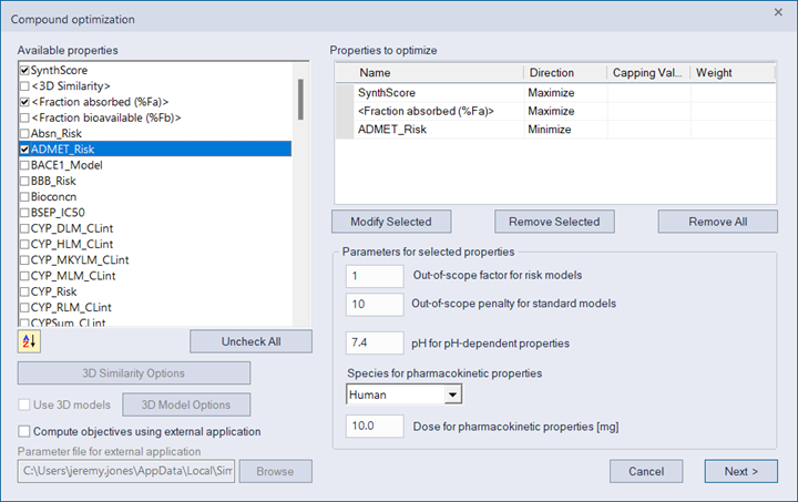
Selecting properties on the left will cause them to appear in the list of Properties to optimize on the right, e.g.:
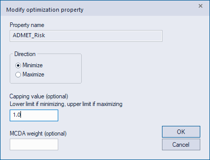
Double clicking on one of the properties in the optimize list (or selecting it and then clicking on Modify Selected) will launch a new dialog Modify optimization property in which one can specify whether the property is to be maximized or minimized and whether to assign a Capping Value and/or the MCDA parameter weight.
Clicking OK will then update the list in the Compound optimization dialog.
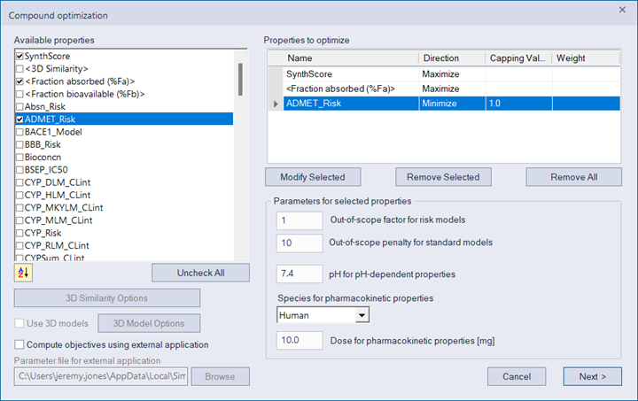
The Capping Value has the following meaning. For an objective that is being maximized and has an assigned Capping Value, if the result of the model calculation is larger than the Capping Value, it is set to that value. Similarly, if the objective is being minimized and its result is less than the Capping Value, its value is set to the Capping Value. The purpose of this parameter is explained in the Theory section of this chapter.
The Weight allows the user to introduce the Multicriteria Decision Analysis weights, which are used in an alternative, MCDA-based pruning scheme. The user can supply the MCDA weight either for all chosen objectives or for none of them. In the former case the MCDA pruning will be applied; in the latter, a default Pareto pruning scenario will be executed. The choice of the pruning method only affects the way the compounds are retained for the next generation.
The Out-of-scope parameters are used to penalize candidate molecules that are in regions of chemical space outside the applicability domain of one of the selected objectives (Properties to optimize). For any standard model (i.e., non-Risk model), the Out-of-scope penalty will be subtracted from or added to the model’s result depending on whether the chosen Property is maximized (subtracted) or minimized (added). The intent is to strongly penalize molecules outside the applicability domain of a given objective so as to reduce the tendency to “wander” into undesirable regions of chemical space. Note that since the penalty is additive, it is best to use models that are built in log-space or whose predictions do not span multiple orders of magnitude. For example, if an activity model is built in “normal” space, it may span a range of 10-3 - 10-9 Molar. A prediction of 10-7 penalized by an additive value of 10 will have no effect when compared to a prediction of 10-6 which is in-scope (inside applicability domain) so that the out-of-scope 10-7 prediction will still be favored (assuming the objective is being minimized). However, in log-space, the prediction of -7 penalized by a value 10 will essentially make this result unfavored against any other reasonable prediction which is in-scope. Note that in the context of AIDD runs, a model is deemed out-of-scope if it or any of its dependent models (Determining descriptors) or its Auxiliary factor is out-of-scope. This is more stringent than the out-of-scope assessment performed during ADMET calculations and helps to further limit the candidate molecules to “reasonable” regions of chemical space.
A separate out-of-scope penalty is used for Risk models. Risk models typically consist of multiple rules invoking multiple models. Assigning a full penalty (e.g. of 10) to a Risk model if any of the models it employs goes out-of-scope turns out to be too strong a penalty and would occur far too often. In this case, the penalty is applied on a per-rule basis in which the weight associated with the rule is multiplied by the out-of-scope factor and added to the Risk score when one of the models employed by that rule goes out-of-scope such that the rule could be triggered if the out-of-scope model’s prediction assumed an “arbitrary” value (i.e., since it’s out-of-scope, we take the conservative view that the true result could trigger the rule). This out-of-scope behavior for Risk rules is a newly added feature as of ADMET Predictor X and is discussed in more detail elsewhere. Note that the default out-of-scope risk factor during ADMET Calculations is set to 0.5 and may be changed in the File >> Preferences >> ADMET tab of the main menu, while in AIDD runs the default is set to 1.0. Setting the Out-of-scope parameters to zero turns off these penalties.
The pH for pH-dependent properties parameter has the same meaning as in the Calculate ADMET dialog and applies to models (S+logD and S+S_pH) that depend on the specified pH. Similarly, pharmacokinetic properties parameters have the same meaning as in the HTPK Simulate fraction absorbed and bioavailable dialog. The pharmacokinetic parameters are only displayed if %Fa or %Fb is selected as one of the objectives.
The Use 3D models check box is used to request that 3D predictive models be calculated, when available. This option is disabled unless all seed compounds have valid 3D atomic coordinates. You can click the 3D Options button to modify the settings for generating 3D coordinates for the virtual compounds.
Since the launch of ADMET Predictor version 10.3, AIDD runs now support the capability to calculate one or more objectives by invoking an external application or program. The total number of objectives counting both internal and external must not exceed 5. Checking on the box to “Compute objectives using external application” will cause AIDD to launch the external application during each generation of compound optimization. Details for informing AIDD how to invoke the external application are contained in the parameter file specified in the “Parameter file for external application” text box. A template for this parameter file, AIDD_ExternalApp_Params.txt, is provided in the user’s \<AppData> folder.
This file contains self-documenting comments that describe a set of keywords and values to be provided describing the specifics of how to invoke the external application for generating external objectives. These keywords include specifications for the name and location of the external program or script to invoke, the name, location, and type of structure file for AIDD to write to supply to the external program (2D SDF or SMILES) and the name and location of the file that the external program will write that will be read by AIDD containing the values of the objectives for each molecule. Other keywords inform AIDD whether a given external objective should be maximized or minimized and whether any internal attributes (e.g., built-in models or descriptors) should be supplied to the external program. Please consult the AIDD_ExternalApp_Params.txt file for full details of the required keywords and their usage.
When AIDD runs in this scenario, it will write a structure file during each generation, launch the external program, wait for it to complete, and then read the results (objectives) from the file written by the external program. After reading the results file, the temporary structure file and results file will be deleted. Users may wish to test usage of the external application by preparing a test structure file that it will read, launching the requisite script or program, and then verifying that the corresponding results file of objective scores has been successfully written.
Beginning with ADMET Predictor 11, users can request an objective representing the 3D similarity to one or more reference conformers. This option makes use of the 3D similarity screening functionality described here. To take advantage of this feature, users must select the objective named \<3D Similarity>, then click the 3D Similarity Options button to specify parameters such as the SD file containing the reference 3D structure(s), the similarity threshold for exporting structure alignments, etc. Note that this feature always results in a single similarity objective; if multiple 3D reference structures are specified, the similarity will represent the maximum of the individual similarity scores.
After selecting the objectives and setting the other parameters on this dialog, click Next to advance to the Filter rules dialog of the AIDD wizard.
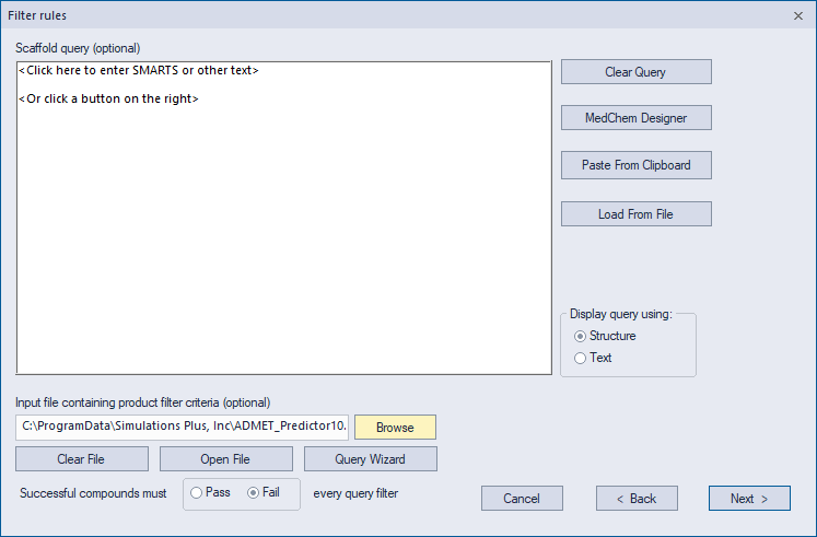
The settings on this dialog are equivalent to those found in the Filter options Dialog which is opened when Add Filters is selected from the Combinatorial Transforms Dialog. In the context of AIDD runs, the Scaffold query is used to define a chemical scaffold that must be present in all candidate molecules generated during an AIDD run, and as mentioned above, this is one way to maintain activity during compound evolution. This is typically used to limit the chemical space that can be explored by candidate molecules. All candidate molecules generated by the SMIRKS transforms must satisfy this query. Any candidate molecule that does not will be immediately rejected without further consideration (i.e., its properties will not be evaluated). Note that if none of the seed molecules (corresponding to the molecules in the selected rows when the AIDD wizard is launched) satisfy this query, the algorithm may be unable to find any candidate molecules satisfying this constraint and will eventually terminate (after trying very hard to find such a molecule) with no results other than the initial seed molecules. It is therefore recommended that the scaffold query be first tested (using the Search using a query dialog) against the seed molecules to ensure that at least some of them satisfy the scaffold requirement.
The Input file containing product filter criteria parameter specifies a file that contains a list of queries that act as filters for each generated candidate molecule. Typically, this will be used to specify a set of chemical functional groups (via SMARTS patterns) that are forbidden in the candidate molecules. ADMET
Predictor offers a default set of such filters in the file, DrugLikeFilters.cqf, which can be found in your application data folder (hereafter termed \<AppData>). Using the default file, all compounds must “fail” every filter, i.e., none of the undesirable SMARTS patterns (functional groups) can be present in any of the generated candidate molecules. Any compound not passing these filters will be immediately rejected without further evaluation.
After optionally specifying a Scaffold query and/or a filters file, selecting Next takes you to the final Dialog of the AIDD wizard, Run parameters.
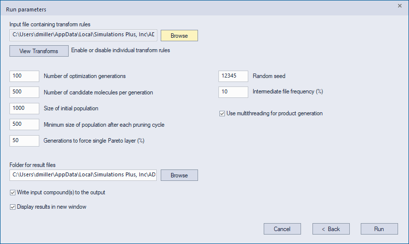
The first parameter, Input file containing transform rules, has the same meaning as the corresponding parameter in the Combinatorial Transform dialog. As discussed in more detail in the Theory section, in AIDD the transforms are not applied combinatorially (with one exception described in the Theory section). Instead, a random molecule is selected from the current population and a random transform is selected from the list of transforms to generate a new candidate molecule which will be evaluated against the objectives if it first passes the Scaffold query and the other filter queries.
The View Transforms button enables the user to turn off individual transforms from the list just as is the case for the Combinatorial Transform feature. With the default Transform file supplied with the program, clicking on View Transforms will produce the following dialog.
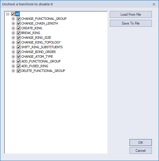
For example, if one wished to exclude iodine from being present in the candidate molecules, first expand the tree under CHANGE_ATOM_TYPE and ADD_FUNCTIONAL_GROUP to view the full list of transforms under the two groupings. Then, uncheck Non-iodine_to_iodine under CHANGE_ATOM_TYPE and Add_iodo under ADD_FUNCTIONAL_GROUP.
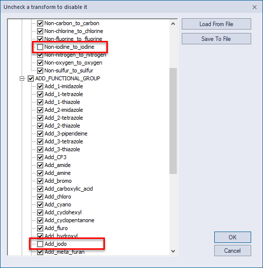
The reason for two transforms, in this case, is that the first replaces a heavy atom with iodine, while the second replaces hydrogen with iodine. This requires two separate SMIRKS transforms. Alternatively, one could include a filter in the filters file that would block iodine. However, excluding it from the Transforms file will yield better performance (shorter run times), since it is more efficient to not generate the product molecule in the first place rather than generating it, testing it against all the filters, and then rejecting it.
The next five parameters on the left side of the Run parameters dialog controls the run-time behavior of the protocol. The algorithm begins by creating an initial population of molecules. All seed molecules are added to the initial population.
No filter checking is performed for the seed molecules. Then, a member of the initial population is selected at random along with a randomly selected transform to generate candidate product molecules which must pass the scaffold and filter queries and are not already present in the population. A given transform along with a starting molecule may generate multiple products. This is explained in more detail in the Theory section. One of the (passing) candidate product molecules is then randomly selected and added to the current population. This procedure is repeated until the size of the initial population reaches the value set by the Size of initial population parameter. This population of molecules is then submitted for ADMET, HTPK, and SynthScore calculations (based on the selected objectives). The population is then pruned to select molecules which are Pareto optimal across the multiple objectives. The Pareto optimal selection process is described in the Theory section. Next, the pruned population is used to generate more candidate molecules by the same procedure involving random selection of a molecule and random selection of a transform. The number of candidate molecules generated for each subsequent generation is controlled by the Number of candidate molecules per generation parameter. These additional candidate molecules are evaluated for their properties, added to the current population, and the current population is pruned again. For example, using default settings, an AIDD run would generate 1000 initial molecules (including the seeds), evaluate their properties, prune the population to be Pareto optimal, generate 500 additional candidate molecules, evaluate their properties, add them to the population and prune again. This protocol will be repeated N times where N is the parameter specified by Number of optimization generations. One finds that from generation to generation, the properties of the population of molecules gradually improves in terms of maximizing or minimizing the target objectives. Finally, the Minimum size of population after each pruning cycle parameter is used to ensure that the population does not become too small after pruning. This requirement is only enforced after the smaller of 100 generations or X% of the total number of generations, where X is defined by the parameter Generations to force single Pareto layer (%). This protocol allows the early populations to grow gradually with “good” molecules.
If pruning in the later stages of the run causes the population to become too small, then additional “layers” of the Pareto surface are selected until the population size reaches the desired minimum. Note that if MCDA pruning is used instead of Pareto pruning, the population size after each pruning cycle is calculated as the product of Minimum size of population after each pruning cycle and the fraction of completed generations. This is explained in more detail in the Theory section.
Since random numbers are used throughout the algorithm, the user may specify a Random seed parameter which is used to initialize the random number sequence. However, specifying the same random seed will not ensure that the same results are obtained for two identical runs (all the same parameters, settings, and initial molecules) unless the Use multithreading for product generation box is unchecked. By default, the algorithm runs multithreaded (i.e., certain operations are performed in parallel) for product generation, ADMET/HTPK calculations, and SynthScore calculations. The number of threads used is specified in File >> Preferences >> Advanced tab by the Maximum number of processors to use for computations setting. When product generation is performed in parallel, candidate product molecules are added from separate threads to the current population in an order which is not reproducible because the addition of each molecule to the current population affects the generation of subsequent molecules. So, in this case, the candidate molecule population may be different, even with the same random number seed. If reproducibility of the results is required, then Use multithreading for product generation should be unchecked. However, this will likely slow down the run by a factor of two or more, depending on other settings (e.g., use of Scaffold query or filter queries).
The Intermediate file frequency (%) parameter specifies how often to write the current molecule population to a file. Depending on the number of generations specified, an AIDD run may take hours or even days. Timings on a modern laptop with an i7-6700 processor running 7 threads with default settings takes ~15-30 minutes per 100 generations. This will vary somewhat depending on the various parameter settings, choice of objectives, etc. The default setting of 100 generations is mainly intended for initial exploratory runs or demos. A full production run to enable the algorithm to approach some kind of convergence may require 1000 or even 10,000 generations. Rather than having to wait until the run completes, intermediate results are written each time the number of current generations reaches a multiple of the Intermediate file frequency (%) times the total number of generations to run. For example, if the Number of optimization generations is 100 and the Intermediate file frequency (%) is 10%, then intermediate results will be output after 10, 20, 30, … 90, 100 generations. The intermediate results are output as a SMILES file with the following columns:
SMILES : the SMILES representation of the compound
ID : a number serving as an identifier. The number represents its overall order in the total list of compounds whose properties were evaluated. Note that when a compound is pruned from the population, then its number will no longer appear.
Generation : The number of the generation in which the molecule was produced.
OBJ_* : A list of objectives with the prefix OBJ_ followed by the name of the objective property. Note that if an objective was “capped” (as a result of having a Capping Value) or is penalized with an out-of-scope penalty that is the value that will be shown, not the “raw” value that results from ADMET/HTPK calculations.
Rxns : A list of reaction ID’s corresponding to the set of reaction transforms that were used to produce this molecule from one of the seed molecules. The reaction names corresponding to the reaction ID’s can be found in the file RxnIDs.txt in the output folder of the AIDD run.
The names of the intermediate files are AIDD_Gen\<nnn>.smi where \<nnn> signifies the generation count corresponding to that instance of the population. By examining the intermediate results file (e.g., in Excel or in another instance of ADMET Predictor), a user may determine that the results have sufficiently converged to Cancel the remainder of the run, or that the intermediate results are undesirable, e.g., exploring undesirable regions of chemical space. In the latter case, the current run may be canceled, and a new run can be initiated with a Scaffold query or filters file designed to block the unwanted chemical moieties. Furthermore, “good” molecules in the intermediate results file can be used as starting seeds for another AIDD run.
The Folder for result files specifies the location where all output files from an AIDD run will be written. These files include the intermediate output files described above, the RxnIDs.txt file, two log files, ADMET_Predictor_Errors.log and AIDD_Run.log, a final results file named AIDD_Results.sdf, and optionally a final file named AIDD_Results_AutoDisplay.ctk. If the option to use an external application was selected, the external application parameters file will also be written to this folder. The ctk file is written if the option Display results in new window is checked on. By default, the results folder is set to \<AppData>\AIDD and each AIDD run will overwrite the results in this folder. A different folder should be selected if you do not wish the results to be overwritten or the files in the current \<AppData>\AIDD folder should be copied or moved elsewhere before initiating a new AIDD run. A description of each of these files follows.
The final ctk and sdf files contain all ADMET (and optionally HTPK if %Fa/%Fb is one of the objectives) results for the final population of molecules along with the additional columns found in the intermediate files described above. In this case, the ADMET/HTPK calculations are not capped or penalized, so they may differ from their corresponding values in the OBJ_ columns. In addition, if a single seed molecule is specified at the beginning and a Scaffold query is also specified, then all molecules in the ctk and sdf files will be depicted such that they are aligned with the common Scaffold. If the option Write input compound(s) to the output is checked on, then all seed molecules will be written to these files as well. All seed molecules are given the identifier Seed_\<original name>. If a given seed molecule is already in the final population, it is only written out once. Seed molecules that did not survive to the final population will have no OBJ_* attributes calculated. Upon opening the ctk file, the Spreadsheet Controls filters are automatically set to filter on the OBJ_* properties.
If Display results in new window is checked on, a new ADMET Predictor instance is launched when the AIDD run is completed (if not canceled) showing the molecules in the ctk file. The reader may wonder why the program outputs two files containing almost the same information. The reason is that ctk files can hold a maximum of 100,000 molecules while no such limit applies to sdf files. In the case of a very long AIDD run with many objectives, the final population might have more than 100,000 molecules and so all the molecules will be present in the sdf file, in this case, while only the first 100,000 will be in the ctk file.
The ADMET_Predictor_Errors.log file lists the ADMET/HTPK parameters used for all ADMET/HTPK runs along with any errors generated for ADMET/HPTK runs for each generation.
The AIDD_Run.log file logs all the AIDD parameters used for this run and reports the state of the population after each generation. It shows the total number of molecules that are kept after pruning in each generation and the number of new molecules added in each generation. After many generations, the population size will tend to stabilize and grow more slowly as it becomes increasingly harder to find new molecules that are Pareto optimal compared to those in the current population. Occasionally, the population may grow smaller from one generation to the next because of the nature of the Pareto optimal pruning algorithm. This is explained in more detail in the Theory section.