

In regression uncertainty analysis, generalized gamma distributions are fitted to the cumulative distributions of squared error and ensemble standard deviation of the training set points. The dashed lines allow you to assess the quality of these fits as well as how accurately they describe the test set. The estimated standard deviation of the predictive error (si,err) is based on the ratio of the respective probability densities as explained in the Theory Section. It can be shown, based on the properties of the cumulative gamma distribution, that the greater the separation between the predicted cumulative squared error distribution and predicted cumulative standard deviation distribution, the stronger is the dependence of the predictive uncertainty on the standard deviation of the submodel predictions. You can get a sense of this dependence by selecting point near the lower left and upper right corners of the plot.
The separation is significant but not large in the sample shown below, which is taken from a model of thermodynamic solubility. This is for a subset of the compounds used to build the commercial model, and in which the test set has been expanded to about 20% for illustrative purposes. Two separate screen captures have been merged to show the differences at the extremes.
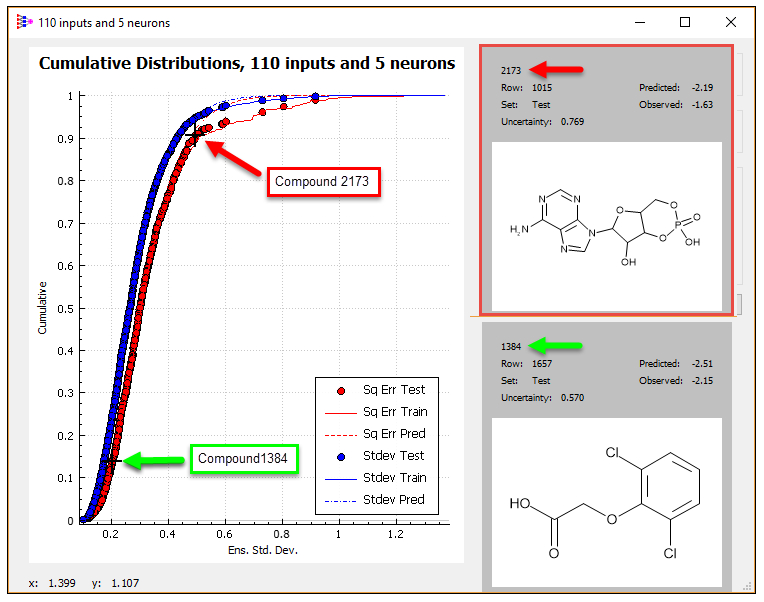
Compound 2173 lies near a break point in the cumulative plot shown above for the Squared Error test set distribution, but the divergence between the observed and predicted statistics is even more evident in the Q-Q Plots shown below. The departure from ideality seems large at first glance, but careful examination shows that appearances are somewhat deceiving in this case. Only a handful of data points in the test set (about 10 of 482, or 2%) fall off the 1:1 line in the Squared Error Q-Q plot. The proportion is similar for the training pool. A similar but somewhat less extreme deviation is evident in the Standard Deviation Q-Q Plots.
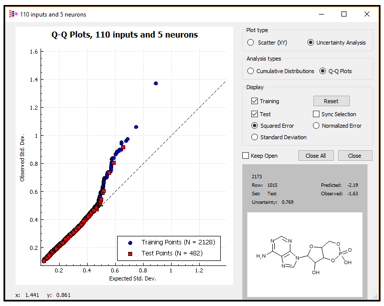
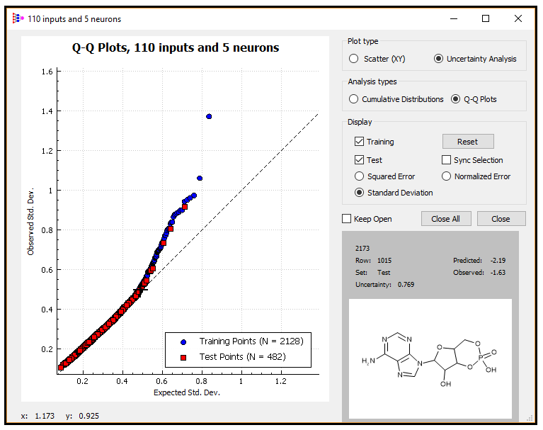
The compounds above the break point include several like 2173 that contain multiple rings and chiral centers, as well as some which form liquid crystals or have very low or very high solubilities. All of these factors make the reported solubilities more prone to experimental error or to misinterpretation or both. Basically, these form a secondary population in the sample used to build the model.
Nonetheless, the Q-Q Plot for the Normalized Error shows good fit across the full range of values. Basically, the deviations noted in the individual fitted distributions cancel each other out in the ratio taken in calculating si,err. in these cases. This indicates that the corresponding uncertainties represented by the error bars shown below can be used with great confidence, even at the extremes of the distribution. It is not a coincidence that the test set RMSE and RMSU are in excellent agreement in for this model.
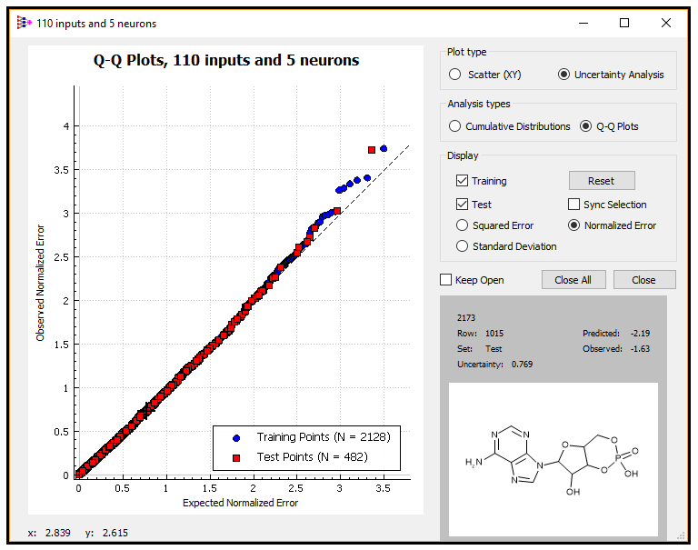
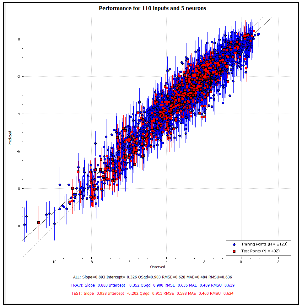
The 110x5 model was ranked fourth in model performance but had the best uncertainty model of the ten models with the best predictive statistics. Even had it not been much simpler than the 110x10 model that ranked highest in the grid, the excellent error model would have been worth the 0.01 to 0.02 sacrifice in RMSE and MAE.