

2.1. What Makes a Good Model?
There are many different things that make a model "good." Building one is very much a multi-objective problem - actually, it is a multi-objective process. This is especially true for the kind of global models we distribute with ADMET Predictor. This chapter lays out some of the things to look for and describes how we provide for those things. Because we use ADMET Modeler to construct our models, there is necessarily some overlap between this section and the ADMET Modeler Chapter How to Build a Good Model. Here we focus more on what you should look for - and look out for - in models built by someone else. Many are things to keep in mind when evaluating software, especially when running comparisons.
Points covered include:
The chapter closes with an anecdote about how models that look too good to be true generally are. For details on one particular validation watch-out and triumph, see the section on CYP Site of Metabolism Models.
Good structures
We spend a lot of time correcting structures in data sets taken from the literature, especially when they come from compilations or some other secondary source. In fact, we usually avoid using any compilation where we are not able to trace a data point back to the original publication.
Sometimes errors are simply a matter of stereochemistry. Mismatches between names and structures are common, especially for metabolites. Incorrect structural isomers are also a problem, most often as relates to compounds being drawn as unrepresentative tautomers, which can cause large predictive errors in some cases. We take pains to train models on dominant tautomers or, where it isn't possible to make that determination unambiguously, reasonably representative ones. The new ADMET Predictor tautomer standardization tool is a good way to do this. Running it on your own data before calculating ADMET properties is a good idea. If you have doubts about the results, it is easy to review them in the pKa Microstates Window.
Good Endpoint Data
For local models, consistency is king: if at all possible, all of your data should come from a single laboratory over a short time period. Barring that, the assay conditions should be as consistent as possible. This does reduce the noise in the data, but it will not be possible to tell how robust your predictions are to small deviations in protocol. It is wise to get data from at least two sources when building a global model. The need to check for consistency in results puts a premium on having reference in common. This is especially true when some data transform is necessary to get endpoint values on a common scale - e.g., [converting IC50 to Ki]. Redundancy in the data actually used to build a model is undesirable, but redundant observations within "raw" data sets and between labs are good because they provides a way to measure how much underlying noise there is in the data.
Broad Applicability Domains
To be useful, a model must have a well-defined "applicability domain," i.e., a way to determine whether a new compound lies within the chemical space over which the model is reasonably valid. This is especially true when regulatory issues are involved and for non-linear models, which tend to extrapolate poorly. Applicability domains for our ANNE models are defined by hypercubes in the model's standardized space: the range of training set values for each descriptor used in the model is mapped to the interval [0,1]. A compound for which any of those descriptors is below -0.1 or above 1.1 is flagged as "out of scope" - i.e., as lying outside the applicability domain of the model. The prediction for such a compound may be correct but it would be unwise to put much faith in it.
Models for which applicability domains are not well-defined should be avoided.
Good Descriptors
In general, we favor property-based descriptors derived from atomic properties over "constitutional" descriptors based on substructure counts. This preference reflects the desirability of having a broad applicability domain. Many of the molecular descriptors used in our proprietary models are derived from properties that reflect the interactions of individual atoms with all other atoms in the molecule. This means that interactions between substructures - e.g., in sulfonylated amidines - can be "covered" by interpolation from nitro, cyano, carbonyl and alkyl substituted analogs. A model based solely on constitutive descriptors, on the other hand, will properly classify such a novel compound as "out of scope."
If the only amidines in a data set bear electron-withdrawing substituents, a prediction for an alkyl analog based solely on constitutive descriptors is likely to be biased even though the compound will not be flagged as "out of scope." A model based on descriptors derived from atomic properties, in contrast, can be expected to detect that the compound lies outside its [applicability domain].
Predictions vs. Table Look-ups
Some ADMET prediction programs are built upon very large compilations of literature data. When presented with a structure for which it already "knows" the answer, such a program can respond in two ways. It can regurgitate the literature value - in which case its "prediction" is likely to be perfect - or it can "hide" the known answer and try to predict it as though it were truly unknown. Returning a look-up value is preferable when the value itself is what matters, but it is misleading when a person is trying to compare predictive performance. The best way to address this problem is to run evaluations using unpublished results, but that is not always practical. A simple but effective alternative is simply to ignore all predictions that are "too good" (error \< 0.05 log units, for example) when compiling performance statistics. If doing so makes a significant difference, you are probably dealing with a look-up model, at least in part.
Protection Against Overtraining
Our models are trained so as to try to maximize their accuracy - i.e., to minimize their error. Usually this is accomplished by minimizing a weighted sum of squared errors. Were that process allowed to go to completion, artificial neural nets (ANNs) and other powerful nonlinear data mining tools models would ultimately produce models with no residual error in predictions for the training set, provided there are no observations with identical descriptors but different response values. The downside of that precise fitting is that the model will likely be unable to accurately predict endpoints for compounds not actually included in the training set.
We protect our ANNs from this risk by testing performance against a companion verification set as part of each cycle of the training process. The error on the training set necessarily decreases or stays the same, but an increase in errors on the verification is a signal that modeling is losing its ability to generalize - i.e., is becoming overfitted. If that continues to be the case over more than a few iterations, the process is stopped "early" and model weights from the stage at which verification performance was optimal is used.
We have no such method for preventing SVM or KPLS overtraining, which is one reason we generally prefer ANNEs.
Unbiased Test Sets
Testing predictive performance on a "held out" test set is the gold standard for validation. We do this by avoiding any opportunity for the dependent variable (endpoint) to bias test set selection. We prefer to use Kohonen mapping or K-means clustering where possible; these stratified sampling techniques examine the data point distribution in the overall descriptor space and generally strike a good balance between making the training pool informative and the test set representative. Neither makes any use of endpoint information in the partitioning process. When data sets are not amenable to either of these methods, we usually turn to stratified sampling, which insures that the dependent variable range is evenly sampled. For many ADMET endpoints of interest, good data is limited, which makes data sets small. The noise introduced by random sampling can easily overwhelm the signal in such cases - it is all too easy to get a misleadingly good or an unnecessarily bad partition by chance - so it is generally better to avoid random sampling unless the data set is large (>1000 examples).
Once selected, the test set does not participate in the model building process; it is only used to assess the performance of the final ensemble model.
Relevant Performance Statistics
We provide several measures of predictive performance for our models. Classification performance is reported in tabular form as training pool and test set [Sensitivity ], the fraction of positive examples that are correctly classified by the model; [Specificity ], the fraction of negatives that are correctly classified; and [Concordance ], the fraction examples that are correctly classified. The number of positive and negative examples is provided to show how (un)balanced each data set is. The degree of imbalance is important because the data sets used to characterize biological activities are often not themselves representative of the population of compounds to which the model will ultimately be applied - i.e., the "target population". This is particularly true for classification models, which are often artificially made more evenly balanced between positive and negative examples than the target population is.
We focus on optimizing specificity and sensitivity because they are insensitive to imbalances in class size. Concordance is quite sensitive to imbalance; optimizing it increases the risk of seeing qualitatively different performance "in the field" than in the test set. Comparing published concordance (or "accuracy") statistics obtained using different data sets should be avoided for this reason.
High sensitivity and high specificity are both good, but there is always a trade-off between the two. Most of our models are optimized by maximizing Youden's index J:
J = Sensitivity + Specificity - 1
which represents an equal weighting of the two performance criteria.
Regression performance is shown in the sections that follow in the form of predicted vs observed plots. Separate summary statistics are presented for the training pool and tests sets; the latter is highlighted in the text because it is typically a better indicator of what you can expect for predictions on novel compounds. Statistics include the root mean square error (RMSE) and mean absolute error (MAE). Typically these are log/log plots, so an RMSE of 0.3 translates to an expected two-fold error range, whereas an RMSE of 0.6 indicates an expected error of about four-fold; the smaller the value, the better the performance.
The slopes and intercepts for the observed vs. predicted regression lines are shown. Perfect agreement between prediction and experiment is indicated by a slope of 1 and an intercept of 0, but it is difficult to assess how meaningful deviations from those values are in any particular case.
The squared Pearson's correlation coefficient (R2) is also reported for regression models. Statistically speaking, this equals the fraction of the variance in y (the observed value) that is explained by x (the predicted value). This statistic is quite sensitive to the range and distribution of values for the dependent variable, just as concordance is sensitive to the degree of imbalance in a categorical data set. It can be a very misleading statistic for comparing model performance on different data sets. RMSE is much better for that purpose.
Confidence Estimates for Individual Predictions
We recently published (Clark 2014) a general methodology for using the degree of consensus between networks in a classification ANNE to accurately estimate the [confidence ]one should have that an individual prediction is correct. This corresponds to the positive and negative predictive value (PPV and NPV) for positive and negative classifications, respectively. Like concordance, confidence estimates are sensitive to the degree of imbalance in a data set.
In doing evaluations against internal or published data, you will need to correct expectations for difference in the degree of imbalance:
Paired Classification and Regression Models
Many ADMET properties - e.g., logP and pKa - can be measured for any compound, at least in principle. For those connected with enzyme or receptor activities - e.g., hERG binding and CYP metabolism - there will be no detectable effect by or on most compounds. Inert compounds do not contribute to regression models and so implicitly fall outside their applicability domains. Creating a classification filter to distinguish substrates from nonsubstrates, as we do for CYP metabolism, is prudent in such cases.
The Model That Looked Too Good to Be True
In originally developing our respiratory model, we turned to a data set of 80 compounds commonly used to model this endpoint. It consists of 40 sensitizers identified through inhalation studies in rats and a balanced subset of 40 of 118 non-sensitizers (Graham 1997). It has subsequently been shown that 80% of the respiratory sensitizers could be assigned to some mechanistic domain (acylation, Michael addition, Schiff base formation, SN2, or SNAr) by applying simple SMARTS rules to classify the compounds (Enoch 2010).
Using the 79 compounds having structural data, ANNC models were built with ADMET Predictor that achieved 100% accuracy using as few as 6 descriptors. Furthermore, a model utilizing a five neurons and a single descriptor was developed that achieved ~90% concordance on the training set. Moreover, it was 100% accurate on the external test set of 8 compounds selected by Kohonen mapping.
The "magic" descriptor was EqualEta, which has a strong reciprocal correlation with molecular weight.
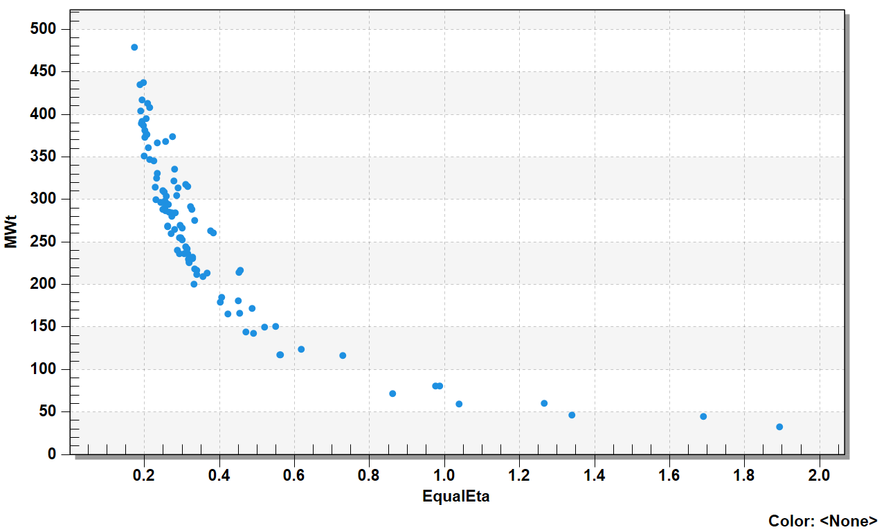
The excessively high performance reflects a high degree of homogeneity within classes ("methyl, ethyl, butyl, futile" syndrome): many of the positives were simple homologous elaborations of each other. As a result, positives that shared a mechanism were similar in size. Any model derived from a "clumpy" data set that small would likely be of little use on any truly external compounds.
Needless to say, we had to expand our data set considerably in order to generate a [Sens_Resp model] that we deemed useful enough to release. You, too, should beware of any such “perfect” model; it is likely to have a very limited (and misleading) applicability domain and to be too good to be true!
A related problem bedevils academic and commercial CYP models that are built from data sets in which every compound is a substrate for some CYP. This implicitly makes any prediction a contingent one - e.g., "This is my prediction assuming that the compound is a substrate for some CYP." Such models almost inevitably over-generalize, classifying all large molecules as CYP3A4 substrates, all bases as substrates for CYP2D6, and all weak acids as CYP2C9 substrates. Moreover, they typically also misclassify those substrates that do not match the corresponding rule-of-thumb archetype. We addressed this for our CYP models by supplementing the data set with large molecules and metabolic intermediates which are demonstrably not CYP substrates.